Temporal Compute · proposed computational laboratory
Less time to a validated result.
A proposed laboratory investigating expensive computation, beginning with high-fidelity path tracing. Quality is a hard constraint; how much of the work is avoidable is the open question.
0.500RMS error · target 0.012
Time ∝ samples. Drag to step through the estimate; switch the objective to move the bar.
Ostrium Labs, Convergence plate, 2026 (illustrative model, canvas, Bayer 4×4 dither)
- Scene
- Analytic sphere and floor; exact answer known
- Noise
- Synthetic, sigma 0.5, falls with the square root of N
- Crossing
- N = (sigma ÷ target)² = 1,737 spp
- Provenance
- Model, not measurement
- State
- Unregistered proposal
- First proposed experiment
- TC-1 · path tracing
- Primary measure
- Time to target quality
- Results
- No published benchmark
The measure · time to target quality Illustrative model · lib/time-to-quality.ts
Time changes the value of computation.
A result is worth having only once it meets its quality contract. Before that, compute buys progress; after it, compute buys almost nothing. The objective is the elapsed time to a validated result, not raw throughput.
Move the target and the deadline. Watch where each method crosses the bar, what the next unit of compute is worth at the deadline, and when a faster method stops counting.
- Uniform sampling
- Reaches the bar at 99 · misses the deadline · marginal value at deadline 1.0e-3 per unit
- Adaptive allocation
- Reaches the bar at 26 · meets the deadline · marginal value at deadline 3.6e-4 per unit
- Compression factor
- 3.8× (uniform time ÷ adaptive time)
Same compute, two allocations. The adaptive one reaches a modest bar several times sooner, but its shortcut leaves a bias that no amount of extra work removes. Raise the target past that floor and it never qualifies, however long it runs. An acceleration that misses the bar does not count. The shapes are assumed; finding where real methods have floors is what a benchmark would have to measure.
Time to target, by target quality
| Target | Uniform sampling | Adaptive allocation | Compression |
|---|---|---|---|
| 0.80 | 24 | 4.0 | 6.0× |
| 0.85 | 43 | 8.3 | 5.2× |
| 0.90 | 99 | 26 | 3.8× |
| 0.93 | 203 | 91 | 2.2× |
| 0.95 | 399 | 494 | 0.8× |
| 0.97 | 1,110 | never | — |
| 0.99 | 9,999 | never | — |
The question, made operable · toy scene Observed · timed on your device
Same bar. Less work?
Time to a target quality, on a scene small enough to have an exact answer. Two ways of spending samples race to the same error bar — timed on your device. Then remove the safeguard and watch the faster method quietly fail.
Scene · exact reference
area light (top) · five slats · the value of a pixel is the fraction of the light it sees
Uniform sampling
- Samples / pixel
- 0
- Error (RMSE)
- —
- Compute time
- 0 ms
- Quality bar
- not yet
Adaptive sampling
- Samples / pixel
- 0
- Error (RMSE)
- —
- Compute time
- 0 ms
- Quality bar
- not yet
Error against samples per pixel on logarithmic axes, for uniform and adaptive sampling, with the quality bar and a slope of one over the square root of N for reference.
Run both strategies. Each keeps sampling until its error against the exact image falls below the bar; the clock counts sampling work, measured in this browser.
The question Temporal Compute proposes to study — time to a target quality — on a scene small enough to have an exact answer. Uniform sampling spends samples everywhere; adaptive sampling spends them where the estimate is still uncertain. The timer counts sampling and the adaptive bookkeeping; the error check against the exact reference is excluded because a real renderer has no exact reference — which is why the proposed TC-1 study fixes its quality measures before measuring. Turn the defensive floor off to see adaptive sampling stall: pixels whose first samples happened to agree are never revisited. A speed-up on this toy says nothing about rendering, AI, CFD or any other workload; Temporal Compute has published no benchmark.
Local identifiers TC-0 and TC-1 belong to this proposal and are separate from the institutional research scales (TC-H … TC-C). No Ostrium benchmark or acceleration has been demonstrated.
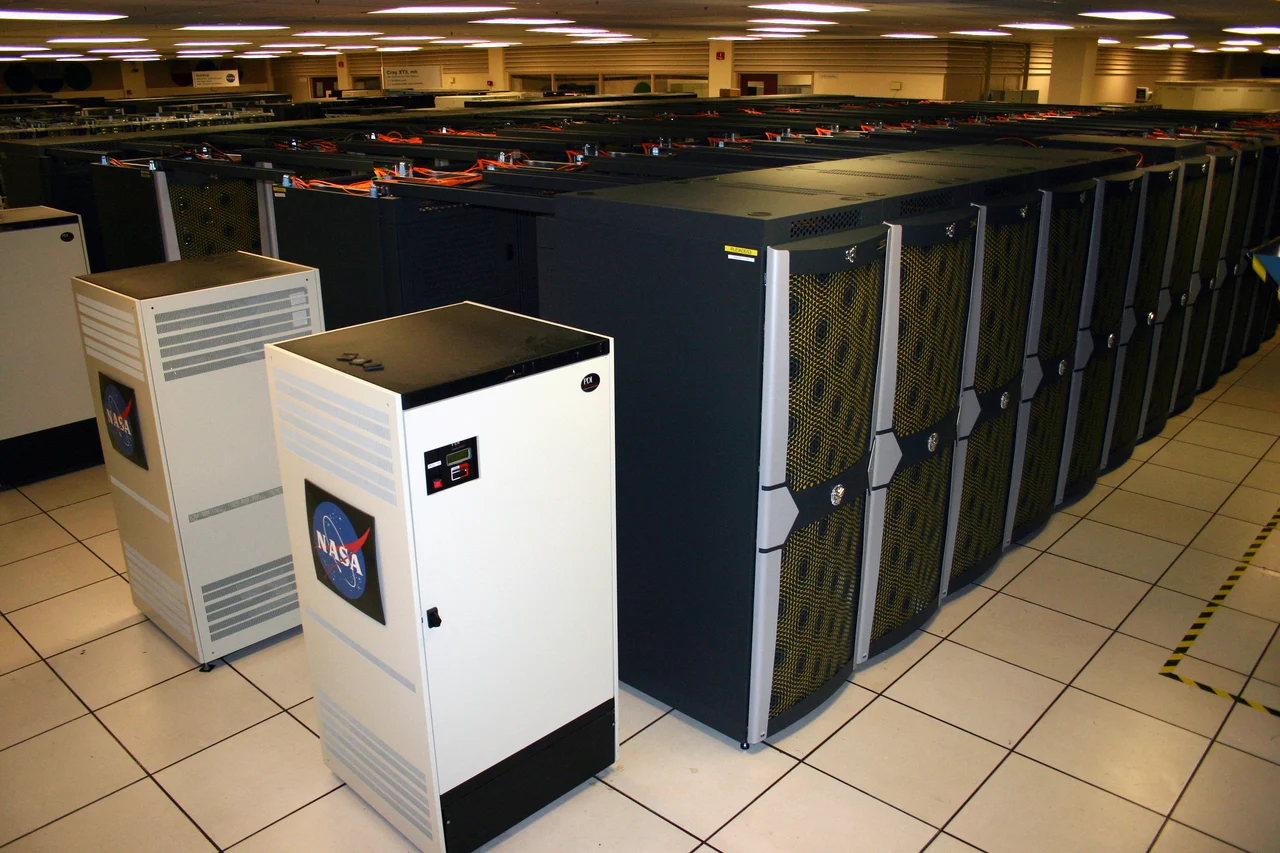
Pleiades at NASA Ames — an external facility, not Ostrium infrastructure. The question is which of this work is necessary to reach an accepted result.
Pleiades supercomputer — Marco Librero, NASA Ames Research Center. Public domain. Resized and encoded as WebP.
The question
Can Ostrium systematically reduce the wall-clock time required to obtain a high-quality computational result?
Temporal Compute is a proposed laboratory for expensive computational workloads. It investigates whether a system can identify useful work, allocate computation where it matters, reuse information, and stop when a defensible quality target is reached.
The objective is time-to-target-quality: the elapsed time from a defined input to a validated useful result. Faster sampling, fewer iterations, or higher GPU throughput are useful only when they improve that end-to-end outcome.
Status: unregistered. This is a project brief and problem definition. There is no published Ostrium benchmark, validated acceleration, implemented general-purpose optimizer, or committed solution architecture associated with this proposal.
The shared computational problem
Different workloads repeatedly spend compute to refine an estimate, search for a candidate, or advance a simulation:
- Path tracing: light paths → radiance estimates → image refinement.
- AI generation: denoising steps → image or video refinement.
- 3D reconstruction: representation updates → scene reconstruction.
- CFD: solver iterations → flow-field estimates → design evaluation.
- Molecular dynamics: force evaluation → timesteps → statistical observables.
- Chip design: candidate layouts → constraint evaluation → revised layouts.
- Compilation: analysis → optimization → code generation → validated build.
These processes do not share one universal convergence criterion. In molecular dynamics, for example, a simulation must preserve the relevant physical statistics; an apparently stable image-style metric cannot establish validity. Each domain needs its own acceptance contract.
The common hypothesis is narrower: some computational latency may be avoidable without changing the task or violating its quality requirements. The amount of avoidable work, the cost of identifying it, and the portability of any method remain unknown.
Objective and marginal compute value
Minimize end-to-end time T, subject to the result meeting the target-quality contract.
For a scalar quality measure where larger is better:
minimize T
subject to Q(result) ≥ Q(target)

Compression factor = T(baseline) / T(candidate)
Marginal compute value = ΔQuality / ΔCompute
Time-based marginal value = [Q(t + Δt) − Q(t)] / Δt
Real acceptance may require several constraints rather than a single Q: numerical error, perceptual fidelity, temporal stability, physical conservation, reproducibility, and resource limits. A prediction of negligible marginal value is a decision to test, not permission to discard rare but important events.
Compression factors must compare the same task, hardware, and acceptance criteria. Prediction, preprocessing, reconstruction, transfer, validation, and failed attempts all contribute to the time budget. A method that merely moves work elsewhere has not demonstrated an end-to-end improvement.
Application domains
Path-traced rendering — first proposed experiment
Problem. Pixels, tiles, materials, and light paths converge unevenly. Difficult indirect illumination, caustics, participating media, tiny bright emitters, and glossy transport can dominate the tail of a render. Other regions may already satisfy the target while continuing to receive samples.
Research opportunities. Measure per-pixel and per-tile convergence; investigate adaptive sample allocation, importance sampling, path guiding, sample reuse, safe path termination, spatial reconstruction, learned denoising, and GPU scheduling. These are candidate directions, not a selected architecture.
Required result. Reach a fixed image-quality target sooner than a competent modern renderer on matched hardware. Preserve geometry, materials, illumination, camera, resolution, and difficult transport. Evaluate numerical and perceptual error together, including localized failures that average scores hide.
Who benefits if it works. Animation and VFX teams, independent artists, architectural and product visualization, renderer developers, render farms, scientific visualization, and synthetic-data pipelines could shorten their feedback loops.
AI image generation
Problem. Repeated denoising and attention computation can make each generation or edit expensive. Fewer steps may change prompt adherence, diversity, composition, or fine detail even when an image looks plausible.
Research opportunities. Study step scheduling, feature caching, token selection, adaptive resolution, region-specific refinement, and stopping criteria. Distinguish inference-time optimizations from methods that require training or distillation; report those costs separately and in amortized totals.
Required result. Shorter time to an accepted image across held-out prompts and seeds, with checks for prompt fidelity, diversity, structure, artifacts, and human preference. A single attractive example is insufficient.
AI video generation
Problem. Space × time produces large token sequences, while repeated denoising compounds compute and memory costs. A shortcut can preserve individual frames while damaging motion, identity, or temporal consistency.
Research opportunities. Investigate progressive resolution, sparse attention, reuse across steps and frames, token and block importance, and targeted refinement. Measure whether the next step improves the accepted video enough to justify its cost.
Required result. Reduce complete generation latency while preserving duration, frame rate, resolution, prompt adherence, motion coherence, and temporal fidelity. Report VRAM, initialization, transfers, and any additional processing.
3D reconstruction / NeRFs
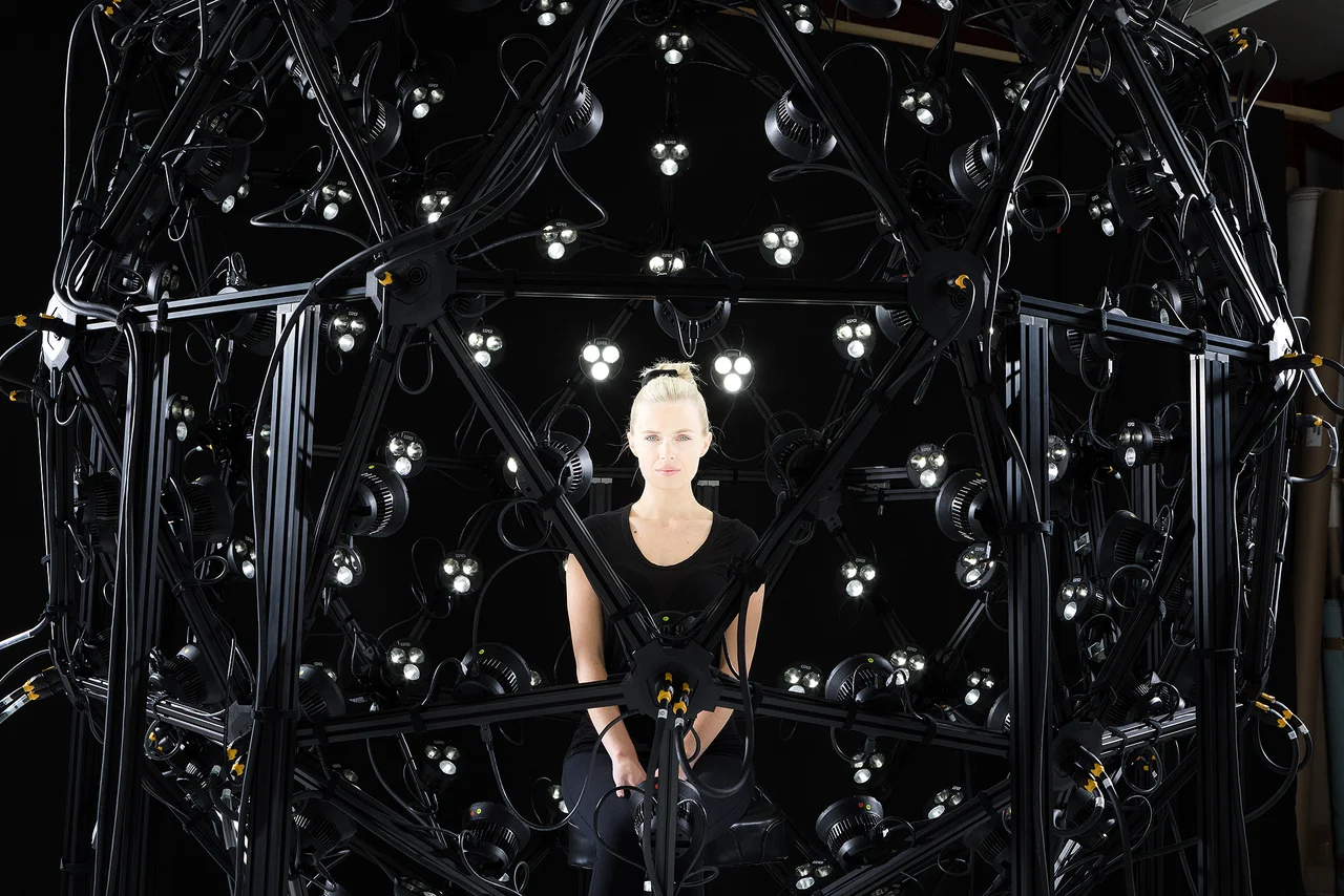
A camera and lighting rig gathers views of a subject. Observations are inputs to reconstruction; this photograph is not a NeRF result or an Ostrium experiment.
Esper LightCage photogrammetry camera rig.jpg — ESPER HQ. CC BY 2.0. Resized and encoded as WebP; image distributed under the stated license.
Problem. Scene optimization repeatedly estimates geometry and appearance from observations. Representation, sampling, memory access, and execution strategy can all affect time to a usable reconstruction.
Research opportunities. Compare scene representations, multiresolution encodings, adaptive ray or view selection, optimized kernels, progressive optimization, and reuse across observations.
Required result. Reach an accepted reconstruction sooner, evaluated on held-out views and geometry where ground truth exists. Include input preparation, training, extraction, and rendering costs. Novel-view image fidelity alone does not establish geometric accuracy.
Chip design / EDA
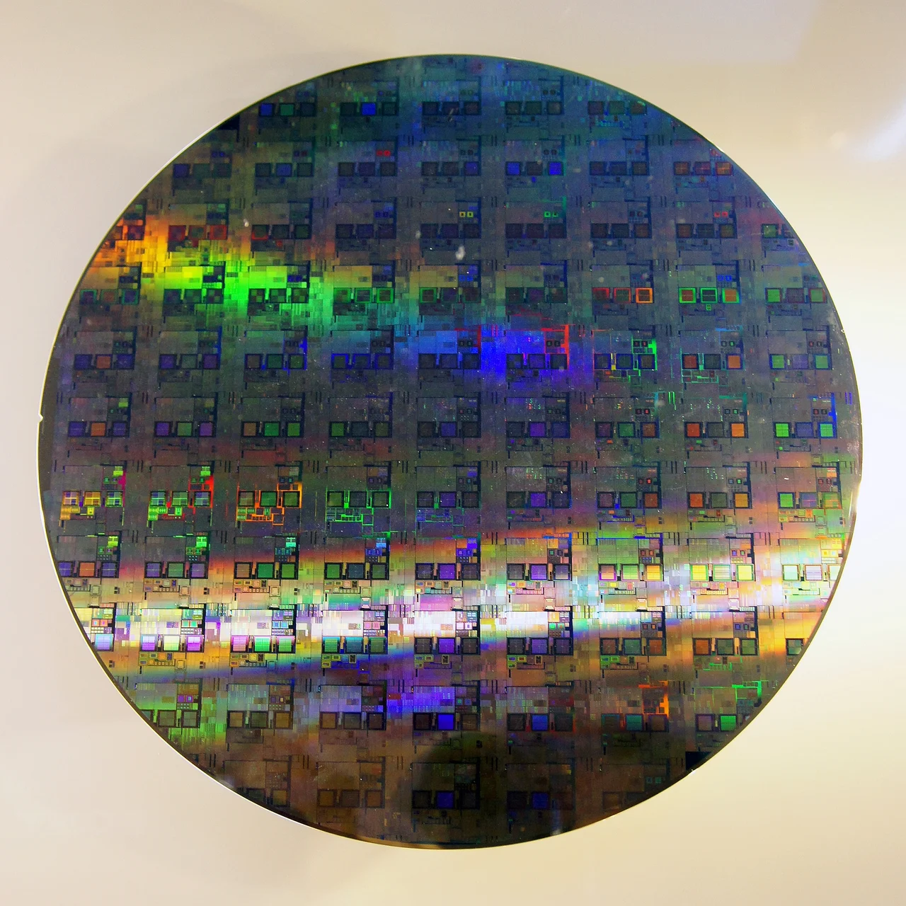
A 12-inch silicon wafer. Chip-design acceleration must ultimately respect physical implementation and verification constraints; the photograph is not an Ostrium design or tapeout.
12-inch silicon wafer.jpg — Peellden. CC BY-SA 3.0. Resized and encoded as WebP; image distributed under the stated license.
Problem. Floorplanning, placement, routing, timing closure, and verification create repeated engineering loops. Improving a proxy score can still leave a design unroutable or unable to meet signoff constraints.
Research opportunities. Explore candidate prioritization, surrogate evaluation, incremental analysis, reusable constraint information, and parallel search. Separate PCB automation from semiconductor physical design; they require different benchmarks and acceptance criteria.
Required result. Reduce time to a feasible, verified design under fixed power, performance, area, timing, and design-rule requirements. Include human intervention and complete verification in the loop-time measurement.
CFD / aerodynamics
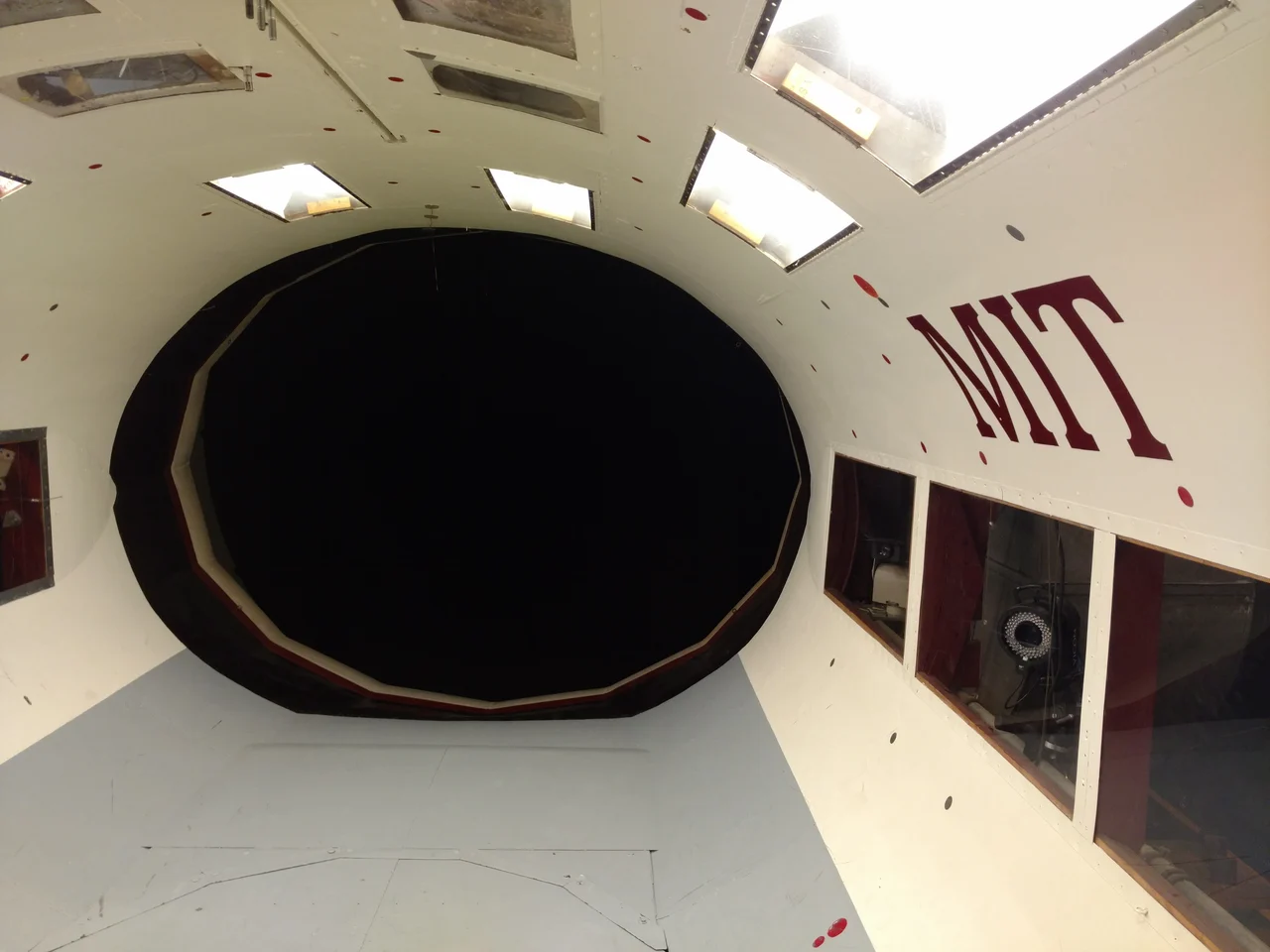
The interior of MIT's Wright Brothers wind tunnel in 2017. Physical testing provides a reference for aerodynamic models; this is a facility photograph, not a CFD flow field.
MIT wind tunnel interior 2017.jpg — Phoebe. CC BY 4.0. Resized and encoded as WebP; image distributed under the stated license.
Problem. Geometry preparation, meshing, numerical solution, and evaluation are repeated during aerodynamic design. Faster solver iterations may not reduce the time to a trustworthy design decision.
Research opportunities. Investigate adaptive meshes, multigrid and solver choices, reduced-order models, surrogate screening, warm starts, and hardware scheduling. Candidate use cases include wings, nozzles, turbines, re-entry bodies, and combustion systems.
Required result. Shorten the geometry → simulation → evaluation → revised geometry loop while preserving accepted error bounds on relevant outputs such as lift, drag, pressure, and heat flux. Check conservation, mesh sensitivity, and agreement with appropriate reference data. A small solver residual alone is insufficient.
Molecular dynamics
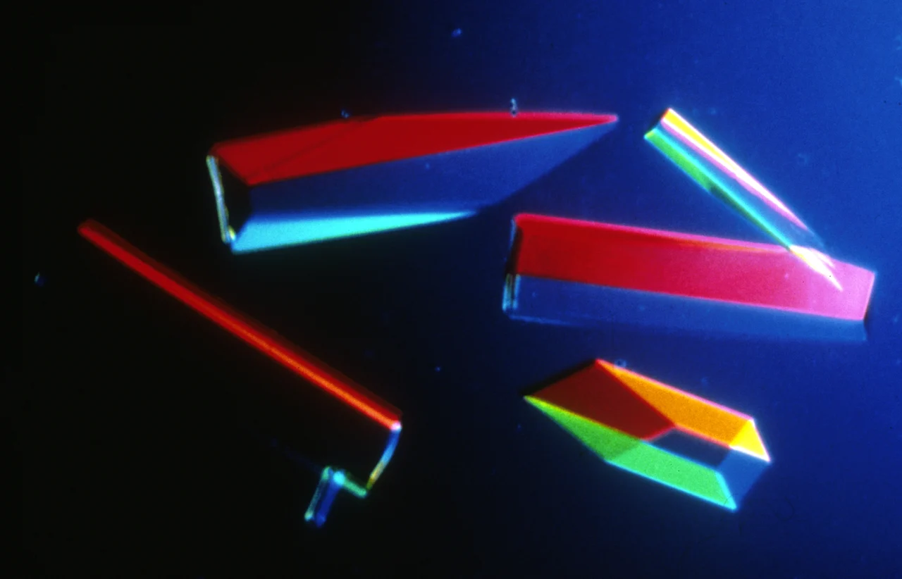
Protein crystals used for X-ray crystallography. Experimental structure can inform molecular research, but a structure photograph does not validate a molecular-dynamics trajectory.
CSIRO ScienceImage 1426 Protein crystals.jpg — division, CSIRO. CC BY 3.0. Resized and encoded as WebP; image distributed under the stated license.
Problem. Long trajectories and repeated force evaluations can make useful statistical observations expensive. Increasing simulated nanoseconds per day does not automatically improve time to a reliable scientific conclusion.
Research opportunities. Study learned potentials, validated surrogate force fields, multiscale models, appropriate timestep adaptation, kernel fusion, distributed execution, and enhanced sampling. Speculative trajectories or region-specific approximations require independent physical validation.
Required result. Reduce time to statistically reliable observables while preserving the relevant ensemble, force accuracy, stability, conservation behavior, and uncertainty estimates. Distinguish a hardware throughput gain from an algorithmic gain and from a change in the physical model.
Compilation and build systems
Problem. Dependency chains, large compilation units, repeated analysis, and cache misses can extend feedback cycles. Parallel work may provide little benefit when a serial critical path dominates.
Research opportunities. Use compilation as an instrumentation exercise: critical-path tracing, incremental rebuilds, caching, parallel execution, and analysis reuse.
Required result. Reduce clean and incremental build latency separately while preserving program semantics, tests, reproducible artifacts, and any required optimization quality. Report cache state, resource use, and the exact toolchain.
Further probes: optimization, robotics, and mission simulation
Candidate extensions include inverse design, materials search, robotic planning, trajectory optimization, and spacecraft mission simulation. Each contains expensive evaluation or search loops that may benefit from better allocation of compute.
These are exploratory horizons. Simulation speed does not establish real-world safety, control authority, or mission readiness. Transfer beyond the first workload requires a new baseline, independent fidelity criteria, and a separately registered experiment.
Why begin with rendering?
Path tracing offers a concrete input, a visible output, controllable repeated runs, mature implementations, and an expensive reference against which to evaluate error. Its sampling process makes the quality–compute–time trade-off observable.
It also provides difficult counterexamples. Rare transport events, temporal flicker, thin geometry, high dynamic range, and denoiser hallucination can expose methods that appear successful on easy scenes. Rendering is a controlled first laboratory; success here would not establish a universal optimization principle.
TC-1: proposed path-tracing protocol
Research question. Where does a render spend time without gaining enough useful information, and can that work be avoided without breaching a defensible quality boundary?
Input contract. A pinned scene, camera, resolution, renderer version, hardware budget, quality thresholds, and random-seed policy. Record geometry, textures, shaders, lighting, integrator settings, and all enabled optimizations.
Baseline. Use Blender Cycles with competent adaptive sampling and denoising settings. A high-sample reference, such as 4,096 samples per pixel, is a candidate starting point rather than a universal ground truth. Confirm reference stability with independent seeds and additional sampling where necessary.
Candidate investigations. Instrument first. Observe sample histories, per-region error, tile completion times, GPU utilization, transfers, memory pressure, reconstruction cost, and validation cost. Only then test convergence prediction, sample budgets, reuse, reconstruction, resolution strategies, or scheduling changes individually.
Scene coverage. Include diffuse surfaces, indirect indoor lighting, many-light scenes, specular and glossy transport, caustics, volumes, subsurface scattering, hair, depth of field, motion blur, small emitters, HDR lighting, and large environments. Separate development scenes from held-out evaluation scenes.
Quality contract. Combine PSNR, SSIM, LPIPS, and FLIP where appropriate, plus localized structural and transport checks and blinded visual review. For animation, evaluate temporal stability. Fix tolerances before measurement; no universal acceptance threshold is asserted in this brief.
Primary measurement. Wall-clock time from the agreed start boundary to an accepted result. For a run that fails the quality contract, report the failure rather than counting it as a fast render.
Secondary measurements. GPU-seconds, energy where measured, peak VRAM, rays traced, samples per pixel, preprocessing and reconstruction time, quality trajectories, tail latency, and run-to-run variability.
Fidelity contract. No hidden change in scene, resolution, light transport, material complexity, hardware, or acceptance criteria. Report cold and warm runs separately. Include predictor overhead and clearly identify training and other one-time costs.
Reporting. Publish scene and software versions, configuration, seeds, repeated-run results, uncertainty, raw quality measurements, failures, ablations, and reproducible commands. Compare against strong existing methods, not only a deliberately oversampled baseline.
Laboratory design
The proposed Temporal Compute Laboratory would observe a workload before attempting to control it:
Workload + baseline + acceptance contract
                  ↓
Instrument time, compute, quality, and memory
                  ↓
Estimate convergence and the value of further work
                  ↓
Allocate / refine / reuse / continue / stop
                  ↓
Independently validate the result
                  ↓
Publish artifacts, measurements, and failures
Potential reusable outputs include a timing harness, dataset manifests, quality evaluators, convergence traces, resource profiles, and benchmark reports. Workload-specific adapters would connect those instruments to renderers or solvers. A general controller should be earned by evidence across workloads rather than assumed at the outset.
Success, failure, and registration gates
Before execution, register the hypothesis, exact measurement boundaries, numerical success threshold, quality tolerances, test-set selection, kill conditions, and cost of reversal. The proposal has not yet met that gate.
Success would mean a reproducible end-to-end time reduction against a competent baseline, on held-out workloads and matched hardware, while every registered fidelity requirement is satisfied. An independent review is needed before any capability claim.
Reasons to stop or narrow the approach include:
- Predictor or reconstruction overhead exceeds the work avoided.
- Gains disappear against an already optimized baseline.
- Quality failures concentrate in rare paths or difficult scene classes.
- Improvements depend on scene-specific tuning or test-set leakage.
- The acceptance metric misses perceptually or physically important errors.
- A method changes the task, shifts costs out of the timer, or relies on undisclosed hardware substitution.
The available record contains no Ostrium results for this project. Numerical examples in the originating brief are illustrations, not experimental measurements. No acceleration factor is promised.
Proposed sequence
TC-0 names the proposed laboratory and its instrumentation work; compilation can be an early systems probe. TC-1 names the first proposed path-tracing experiment. These local identifiers do not replace Ostrium’s institutional TC-H, TC-T, TC-O, TC-D, and TC-C research scales.
The suggested sequence is instrumentation → path tracing → image generation → video generation → 3D reconstruction → scientific simulation. CFD and molecular dynamics each require their own validation infrastructure. EDA is a parallel candidate domain; mission and trajectory simulation remain longer-horizon probes.
Advancement depends on reusable artifacts and evidence from the preceding work. This sequence is a research direction, not a delivery schedule or a claim that all domains admit the same method.
Prior work and evidence boundaries
The brief is motivated by existing optimization work. These sources demonstrate particular methods under their own experimental conditions; they do not establish Ostrium’s hypothesis or predict its speedup.
- Blender Cycles sampling documentation: baseline controls for sampling, adaptive allocation, and denoising. TC-1 must account for capabilities the renderer already provides.
- Instant Neural Graphics Primitives, NVIDIA, 2022: multiresolution hash encoding and fused CUDA execution show how representation and implementation can alter the cost of neural graphics. This is a workload-specific precedent.
- Jenga: Training-Free Efficient Video Generation via Dynamic Token Carving, 2025: progressive resolution and dynamic attention allocation provide a precedent for varying computation across diffusion stages. Its reported evaluation is external evidence, not an Ostrium benchmark.
The foundational question for this project remains open: how much work can be removed before the result stops meeting the contract?